Catherine Kim, PhD
Technology Trainer, The University of Queensland Library
Prerequisites
This R workshop assumes basic knowledge of R including:
- Installing and loading packages
- How to read in data
- read.csv
- read_csv
- and similar
- Creating objects in R
We are happy to have any and all questions though!
What are we going to learn?
In the second part of this workshop, we will learn how to:
- convert to time series objects
- investigate aspects of a times series such as trends, seasonality, and stationarity
- assess autocorrelation
- apply different models
Load packages
library(tidyverse)
library(lubridate) # work with date/time data
library(readxl) # read excel files

library(zoo)
library(forecast)
library(tseries) # test for stationarity
About the data
Sampling design: Atmospheric samples of the Compound X were collected each day during seven consecutive days for different month in the year. Some year and months had less samples due to technical problems.
Read in the data
For this section, we will go the process of analysing time series for one site.
Let’s read in the cleaned data from Part 1, filter out the same site (1335), and split the Date column with lubridate. This can be done in one go with piping.
s1335 <- read_csv("data/analytes_data_clean.csv") %>%
   filter(Site == "1335") %>%
   mutate(Year = year(Date),
          Month = month(Date),
          Day = day(Date),
          Site = factor(Site)) # change Site to a factor
## Rows: 720 Columns: 4
## -- Column specification --------------------------------------------------------
## Delimiter: ","
## chr  (1): Analyte
## dbl  (2): Site, mg_per_day
## date (1): Date
##
## i Use `spec()` to retrieve the full column specification for this data.
## i Specify the column types or set `show_col_types = FALSE` to quiet this message.
s1335
## # A tibble: 352 x 7
##    Site  Analyte Date       mg_per_day  Year Month   Day
##    <fct> <chr>   <date>          <dbl> <dbl> <dbl> <int>
##  1 1335  x       1991-11-28      0.253  1991    11    28
##  2 1335  x       1991-11-29      0.239  1991    11    29
##  3 1335  x       1991-11-30      0.197  1991    11    30
##  4 1335  x       1991-12-01      0.173  1991    12     1
##  5 1335  x       1991-12-02      0.222  1991    12     2
##  6 1335  x       1991-12-03      0.191  1991    12     3
##  7 1335  x       1992-01-30      0.298  1992     1    30
##  8 1335  x       1992-01-31      0.253  1992     1    31
##  9 1335  x       1992-02-01      0.256  1992     2     1
## 10 1335  x       1992-02-02      0.284  1992     2     2
## # ... with 342 more rows
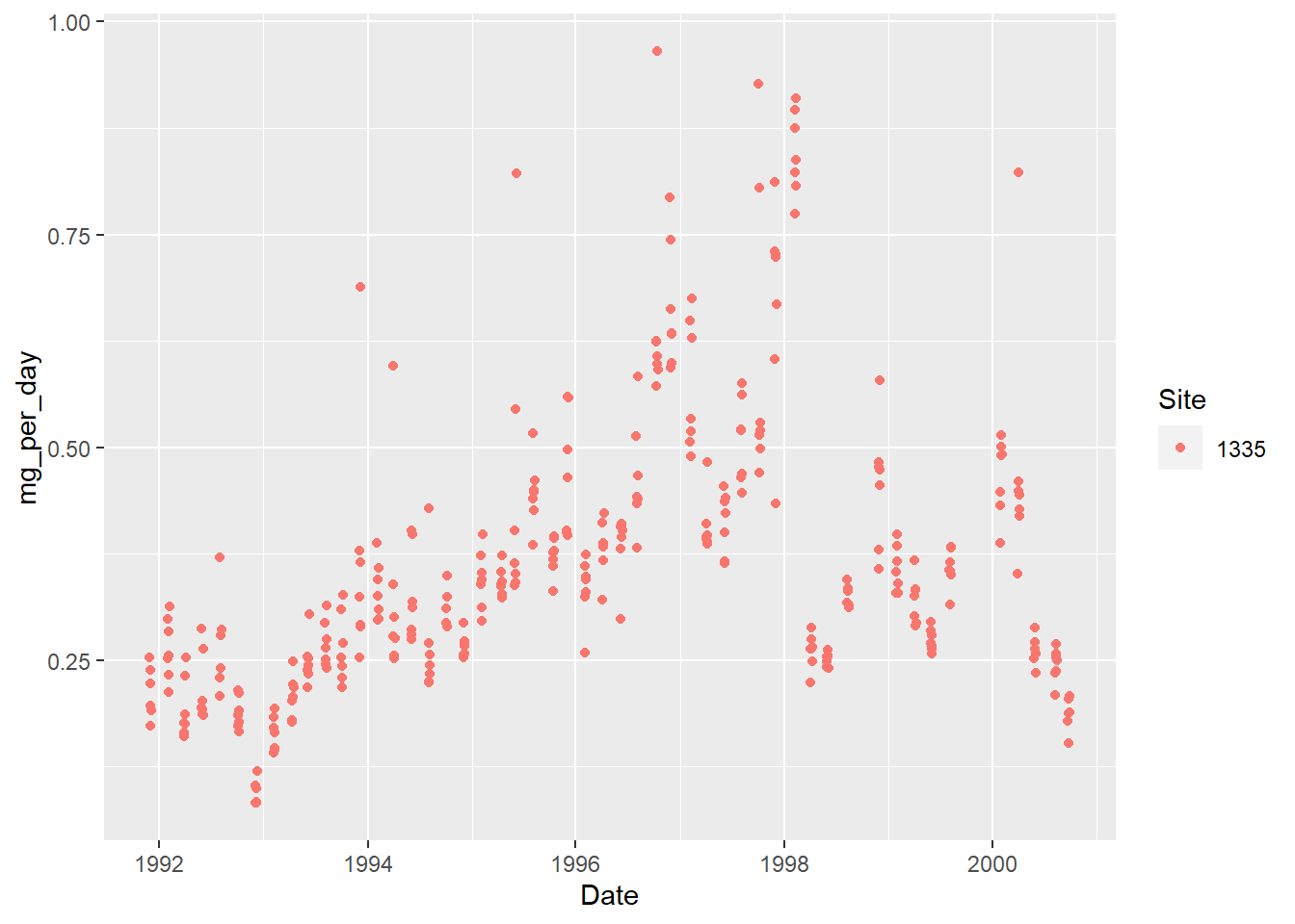
Visualize the data for one site
ggplot(s1335,
        aes(Date, mg_per_day, color = Site)) +
   geom_point()
Count the number of samples per month.
s1335 %>%
   group_by(Year, Month) %>%
   summarize(count = n()) %>%
   arrange(-count) # arrange by count column in descending order
## `summarise()` has grouped output by 'Year'. You can override using the `.groups` argument.
## # A tibble: 68 x 3
##     Year Month count
##    <dbl> <dbl> <int>
##  1  1992    10     7
##  2  1993     2     7
##  3  1993     4     7
##  4  1993     6     7
##  5  1993     8     7
##  6  1993    12     7
##  7  1994     2     7
##  8  1994     6     7
##  9  1994     8     7
## 10  1994    12     7
## # ... with 58 more rows
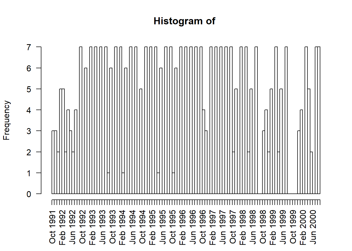
The maximum number of samples we have per month is 7. Probably not enough to do any meaningful analysis for a daily trend. Let’s average samples by month. There also can be no data gaps for a time series (ts) data class.
ave_s1335 <- s1335 %>%
   group_by(Year, Month, Site) %>%
   summarize(mg_per_day = mean(mg_per_day),
             SD = sd(mg_per_day))
## `summarise()` has grouped output by 'Year', 'Month'. You can override using the `.groups` argument.
Alternatively, can graphically summarize the distribution of dates using the hist() (hist.Date()) function.
hist(as.Date(s1335$Date), # change POSIXct to Date object
     breaks = "months",
     freq = TRUE,
     xlab = "", # remove label so doesn't overlap with date labels,
     format = "%b %Y", # format the date label, mon year
     las = 2)
Let’s convert our data into a time series. Times series data must be sampled at equispaced points in time.
There are several different time series object that have different functionalities such as working with irregularly spaced time series. See this resource.
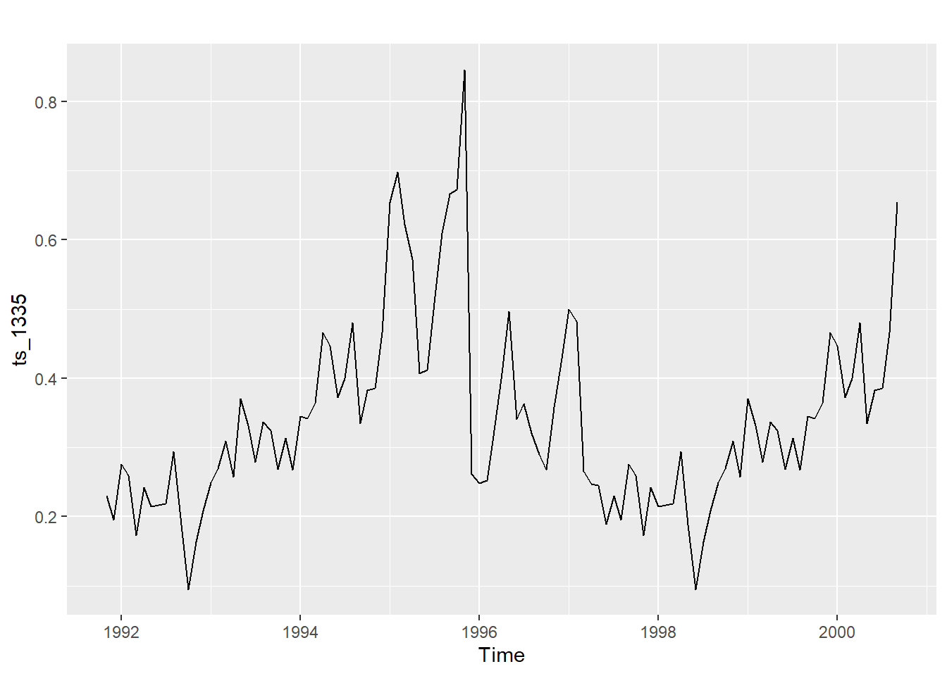
ts_1335 <- ts(ave_s1335$mg_per_day, frequency = 12,
                 start = c(1991, 11), end = c(2000, 9))

class(ts_1335) # check the object class
## [1] "ts"
ts_1335 # see the data
##             Jan        Feb        Mar        Apr        May        Jun
## 1991
## 1992 0.27545325 0.25955623 0.17283015 0.24237330 0.21492034 0.21685501
## 1993 0.24936087 0.26921357 0.30978222 0.25693728 0.37014955 0.33177930
## 1994 0.34481141 0.34235679 0.36426187 0.46659618 0.44669432 0.37206745
## 1995 0.65457749 0.69834479 0.62221301 0.57168051 0.40724687 0.41195379
## 1996 0.24812201 0.25220778 0.32420921 0.40677658 0.49618890 0.34124538
## 1997 0.49926914 0.48207736 0.26538307 0.24687993 0.24478730 0.18937818
## 1998 0.21492034 0.21685501 0.21884272 0.29415920 0.18834451 0.09494631
## 1999 0.37014955 0.33177930 0.27831867 0.33660285 0.32467068 0.26865238
## 2000 0.44669432 0.37206745 0.39990788 0.47986144 0.33436319 0.38241556
##             Jul        Aug        Sep        Oct        Nov        Dec
## 1991                                             0.22975903 0.19544291
## 1992 0.21884272 0.29415920 0.18834451 0.09494631 0.16351067 0.20807004
## 1993 0.27831867 0.33660285 0.32467068 0.26865238 0.31360895 0.26773691
## 1994 0.39990788 0.47986144 0.33436319 0.38241556 0.38570498 0.46601276
## 1995 0.50863024 0.60921090 0.66656370 0.67302314 0.84627446 0.26116715
## 1996 0.36344698 0.32072347 0.29003143 0.26723167 0.35837799 0.42259062
## 1997 0.22975903 0.19544291 0.27545325 0.25955623 0.17283015 0.24237330
## 1998 0.16351067 0.20807004 0.24936087 0.26921357 0.30978222 0.25693728
## 1999 0.31360895 0.26773691 0.34481141 0.34235679 0.36426187 0.46659618
## 2000 0.38570498 0.46601276 0.65457749
Create a irregularly spaced time series using the zoo (Zeileis ordered observations) package
The zoo class is a flexible time series data with an ordered time index. The data is stored in a matrix with vector date information attached. Can be regularly or irregularly spaced. See this document.
library(zoo)
z_1335 <- zoo(s1335$mg_per_day, order.by = s1335$Date)

head(z_1335)
## 1991-11-28 1991-11-29 1991-11-30 1991-12-01 1991-12-02 1991-12-03
##  0.2530688  0.2390078  0.1972005  0.1728767  0.2224569  0.1909951
Decomposition
Decomposition separates out a times series \(Y_{t}\) into a seasonal \(S_{t}\), trend \(T_{t}\), and error/residual \(E_{t}\) components. NOTE: there are lot of different words for this last component - irregular, random, residual, etc. See resources at the bottom.
These elements can be additive when the seasonal component is relatively constant over time.
$$Y_{t} = S_{t} + T_{t} + E_{t}$$
Or multiplicative when seasonal effects tend to increase as the trend increases.
$$Y_{t} = S_{t} * T_{t} * E_{t}$$
The decompose() function uses a moving average (MA) approach to filter the data. The window or period over which you after is based on the frequency of the data. For example, monthly data can be averaged across a 12 month period. Original code from Time Series Analysis with R Ch. 7.2.1.
library(xts)
##
## Attaching package: 'xts'
## The following objects are masked from 'package:dplyr':
##
## first, last
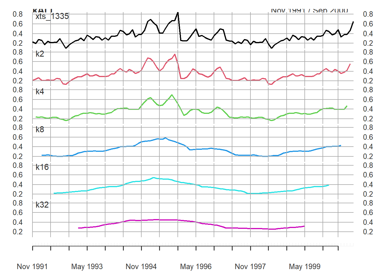
xts_1335 <- as.xts(x = ts_1335)
k2 <- rollmean(xts_1335, k = 2)
k4 <- rollmean(xts_1335, k = 4)
k8 <- rollmean(xts_1335, k = 8)
k16 <- rollmean(xts_1335, k = 16)
k32 <- rollmean(xts_1335, k = 32)
kALL <- merge.xts(xts_1335, k2, k4, k8, k16, k32)
head(kALL)
## xts_1335 k2 k4 k8 k16 k32
## Nov 1991 0.2297590 0.2126010 NA NA NA NA
## Dec 1991 0.1954429 0.2354481 0.2400529 NA NA NA
## Jan 1992 0.2754533 0.2675047 0.2258206 NA NA NA
## Feb 1992 0.2595562 0.2161932 0.2375532 0.2258988 NA NA
## Mar 1992 0.1728301 0.2076017 0.2224200 0.2245342 NA NA
## Apr 1992 0.2423733 0.2286468 0.2117447 0.2368738 NA NA
plot.xts(kALL, multi.panel = TRUE)
Let’s use the use the stats::decompose() function for an additive model:
decomp_1335 <- decompose(ts_1335, type = "additive") # additive is the default
plot(decomp_1335)
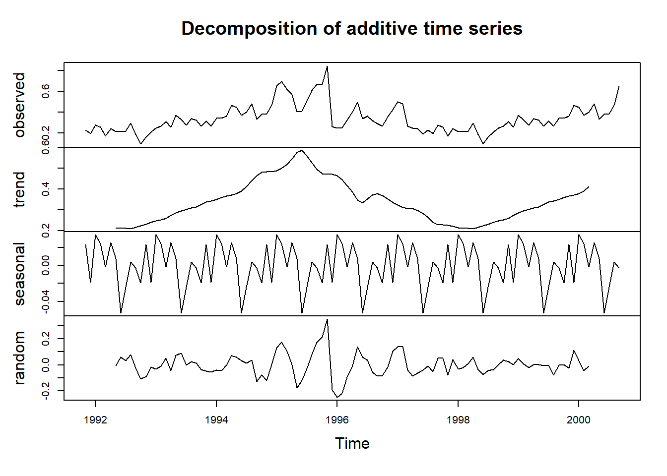
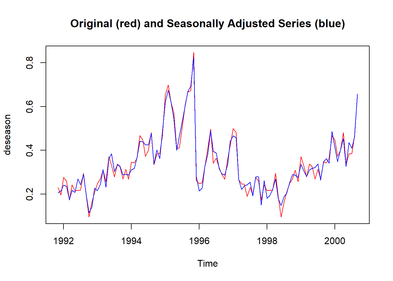
In the top ‘observed’ plot there does not appear to be a clear case of seasonality increasing over time so the additive model should be fine. There is a huge peak in the trend in 1995 which decreases until around 1998 before increasing again.
Remove seasonality components using the forecast package.
stl_1335 <- stl(ts_1335, s.window = "periodic") # deompose into seasonal, trend, and irregular components
head(stl_1335$time.series)
##              seasonal     trend    remainder
## Nov 1991  0.021512597 0.2253694 -0.017122969
## Dec 1991 -0.019995577 0.2243884 -0.008949903
## Jan 1992  0.035564624 0.2234074  0.016481258
## Feb 1992  0.024725533 0.2220857  0.012744950
## Mar 1992 -0.007203528 0.2207641 -0.040730440
## Apr 1992  0.028745667 0.2191495 -0.005521904
The seasonal and reminder/irregular components are small compared to the trend component.
Let’s seasonally adjust the data and plot the raw data and adjusted data.
sa_1335 <- seasadj(stl_1335) # seasonally adjusted data

par(mfrow = c(2,1))
plot(ts_1335) #, type = "1")
plot(sa_1335)
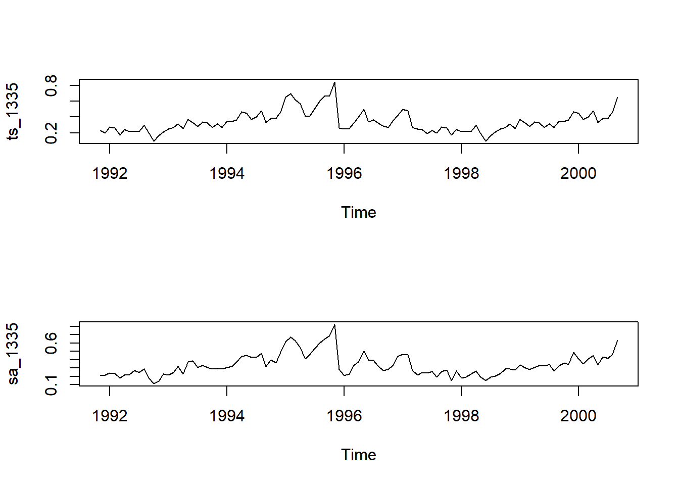
These two plots are pretty much the same. There does not seem to be a large seasonality component in the data.
It can also be visualised using on the same plot to highlight the small effect of seasonality. Code modified from Time Series Analysis with R Ch. 7.3.
s1335_deseason <- ts_1335 - decomp_1335$seasonal # manually adjust for seasonality

deseason <- ts.intersect(ts_1335, s1335_deseason) # bind the two time series

plot.ts(deseason,
        plot.type = "single",
        col = c("red", "blue"),
        main = "Original (red) and Seasonally Adjusted Series (blue)")
Plot the time series against the seasons in separate years.
par(mfrow = c(1,1))
seasonplot(sa_1335, 12,
           col = rainbow(12),
           year.labels = TRUE,
           main = "Seasonal plot: Site 1335")
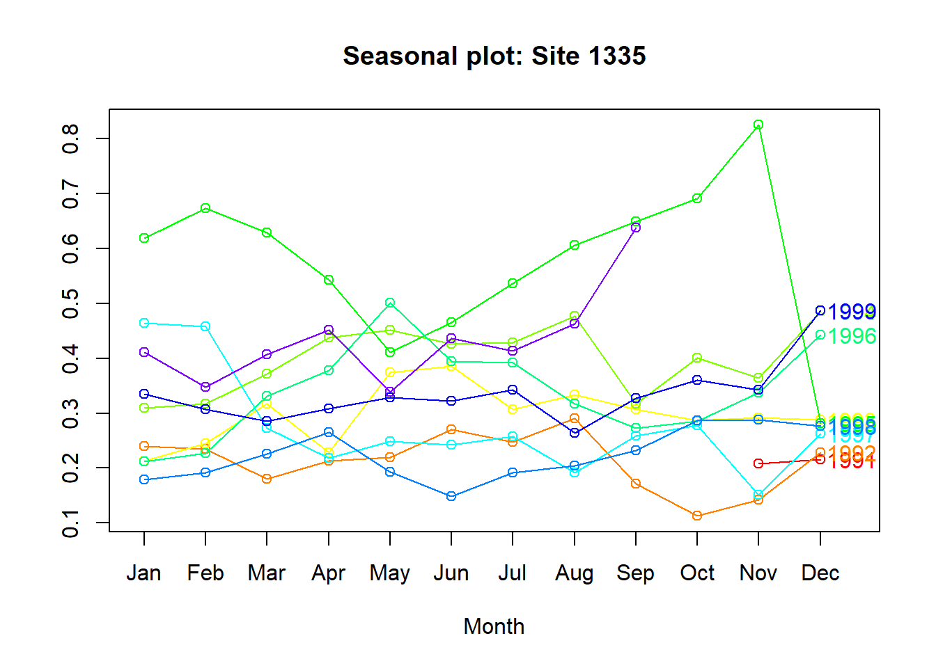
The lines do not really follow the same pattern throughout the year - again, not a big seasonality component.
Stationarity
The residual part of the model should be random where the model explained most significant patterns or signal in the time series leaving out the noise.
This article states that the following conditions must be met:
- The mean value of time-series is constant over time, which implies, the trend component is nullified.
- The variance does not increase over time.
- Seasonality effect is minimal.
There are a few tests for stationarity with the tseries package: Augmented Dickery-Fuller and KPSS. See this section.
adf.test(ts_1335) # p-value < 0.05 indicates the TS is stationary
##
## 	Augmented Dickey-Fuller Test
##
## data:  ts_1335
## Dickey-Fuller = -2.0988, Lag order = 4, p-value = 0.5357
## alternative hypothesis: stationary
kpss.test(ts_1335, null = "Trend") # null hypothesis is that the ts is level/trend stationary, so do not want to reject the null, p > 0.05
## Warning in kpss.test(ts_1335, null = "Trend"): p-value smaller than printed p-
## value
##
## 	KPSS Test for Trend Stationarity
##
## data:  ts_1335
## KPSS Trend = 0.25335, Truncation lag parameter = 4, p-value = 0.01
The tests indicate that the time series is not stationary. How do you make a non-stationary time series stationary?
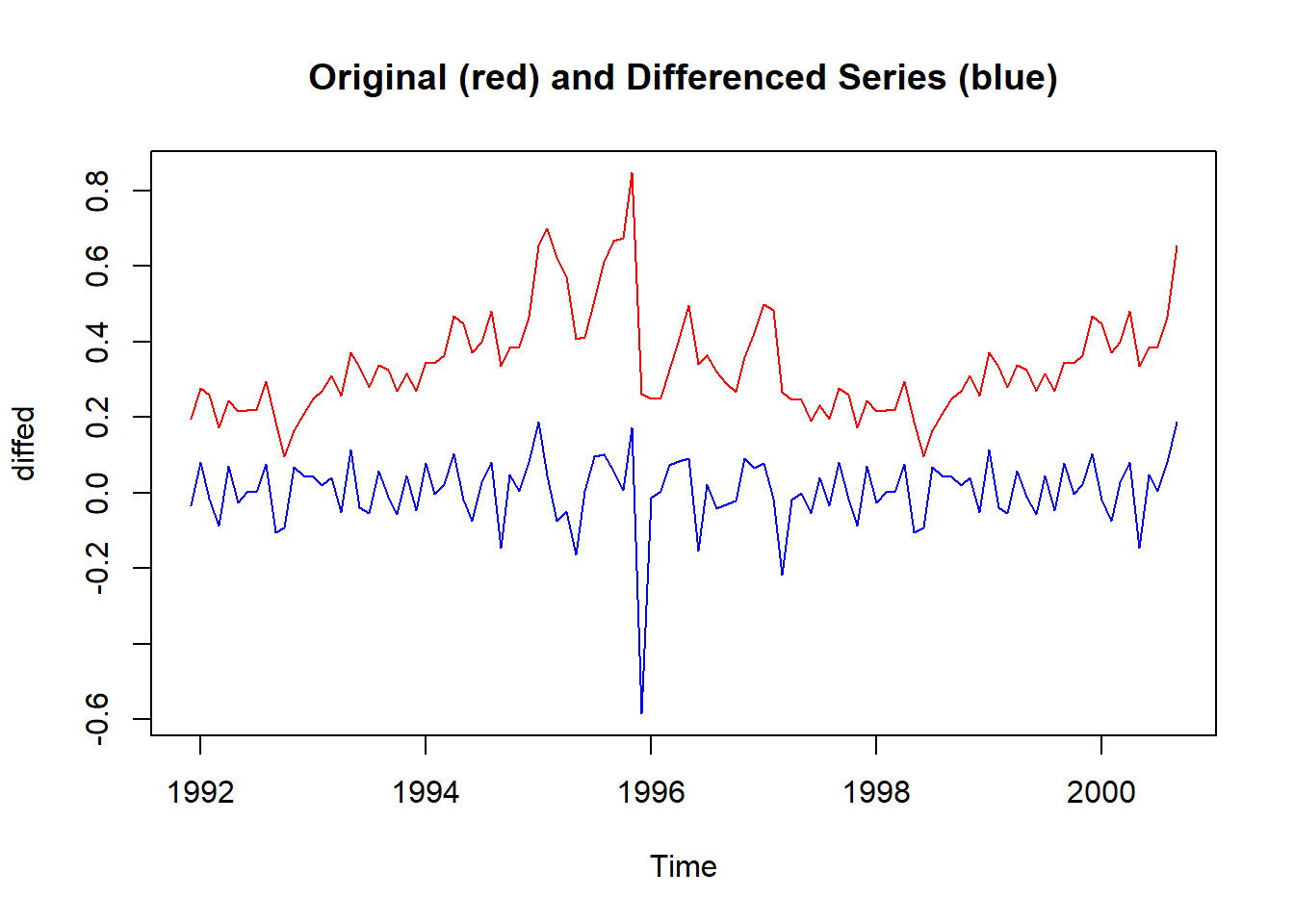
Differencing
One common way is to difference a time series - subtract each point in the series from the previous point.
Using the forecast package, we can do seasonal differencing and regular differencing.
nsdiffs(ts_1335, type = "trend") # seasonal differencing
## Warning: The chosen seasonal unit root test encountered an error when testing for the first difference.
## From seas.heuristic(): unused argument (type = "trend")
## 0 seasonal differences will be used. Consider using a different unit root test.
## [1] 0
ndiffs(ts_1335, type = "trend") # type 'level' deterministic component is default
## [1] 1
stationaryTS <- diff(ts_1335, differences= 1)

diffed <- ts.intersect(ts_1335, stationaryTS) # bind the two time series

plot.ts(diffed,
        plot.type = "single",
        col = c("red", "blue"),
        main = "Original (red) and Differenced Series (blue)")
Let’s check the differenced time series with the same stationarity tests:
adf.test(stationaryTS)
## Warning in adf.test(stationaryTS): p-value smaller than printed p-value
##
## 	Augmented Dickey-Fuller Test
##
## data:  stationaryTS
## Dickey-Fuller = -8.1769, Lag order = 4, p-value = 0.01
## alternative hypothesis: stationary
kpss.test(stationaryTS, null = "Trend")
## Warning in kpss.test(stationaryTS, null = "Trend"): p-value greater than printed
## p-value
##
## 	KPSS Test for Trend Stationarity
##
## data:  stationaryTS
## KPSS Trend = 0.069269, Truncation lag parameter = 4, p-value = 0.1
The both tests now indicate the differenced time series is now stationary.
Autocorrelation
Autocorrelation plots
Plot the autocorrelation function (ACF) correlogram for the time series. There are k lags on the x-axis and the unit of lag is sampling interval (month here). Lag 0 is always the theoretical maximum of 1 and helps to compare other lags.
The cutest explanation of ACF by Dr Allison Horst:
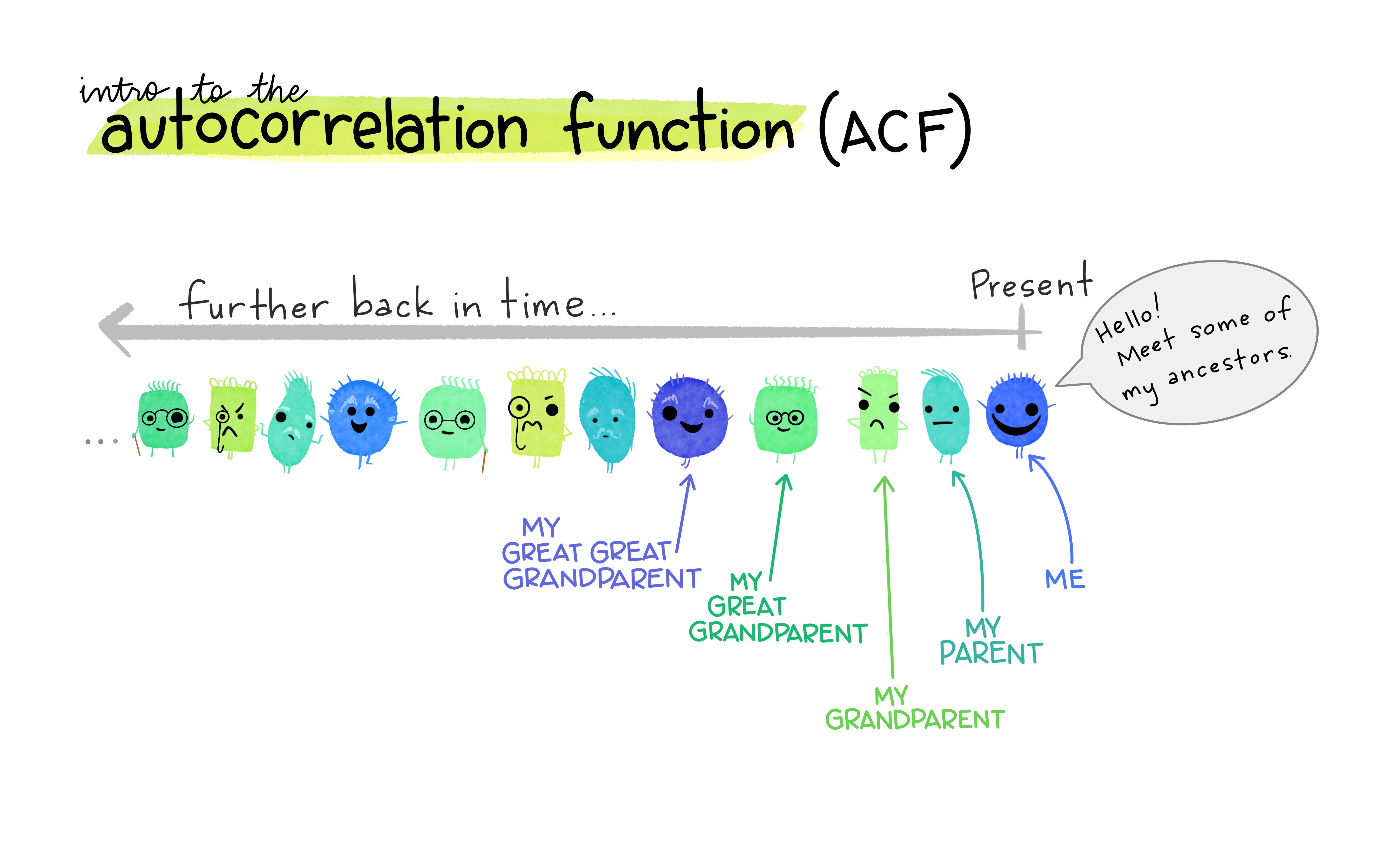
See the full artwork series explaining ACF here.
acf(s1335$mg_per_day)
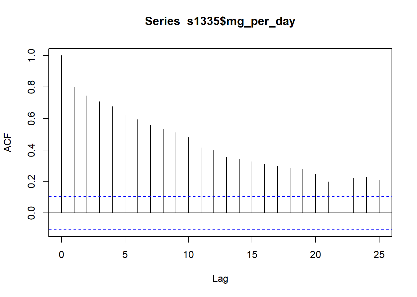
You can used the ACF to estimate the number of moving average (MA) coefficients in the model. Here, the number of significant lags is high. The lags crossing the dotted blue line are statistically significant.
The partial autocorrelation function can also be plotted. The partial correlation is the left over correlation at lag k between all data points that are k steps apart accounting for the correlation with the data between k steps.
pacf(s1335$mg_per_day)
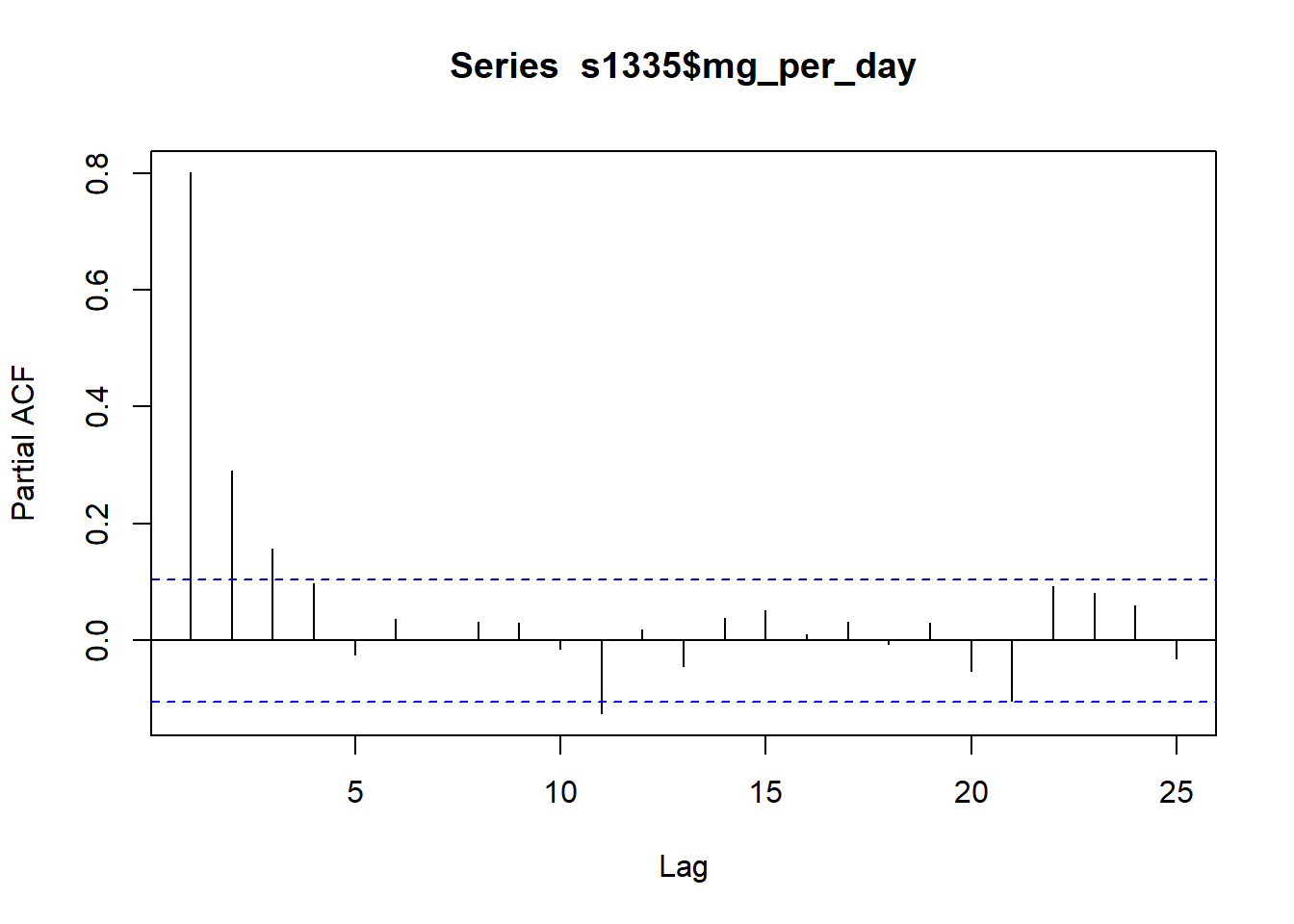
Practically, this can help us identify the number of autoregression (AR) coefficients in an autoregression integrated moving average (ARIMA) model. The above plot shows k = 3 so the initial ARIMA model will have three AR coefficients (AR(3)). The model will still require fitting and checking.
Autocorrelation test
There is also the base::Box.test() function that can be used to test for autocorrelation:
Box.test(ts_1335)
##
## 	Box-Pierce test
##
## data:  ts_1335
## X-squared = 57.808, df = 1, p-value = 2.887e-14
The p-value is significant which means the data contains significant autocorrelations.
Models for time series data
Most of the content below follows the great book: Introductory Time Series with R by Cowpertwait & Metcalfe.
Autoregressive model
Autoregressive (AR) models can simulate stochastic trends by regressing the time series on its past values. Order selection is done by Arkaike Information Criterion (AIC) and method chosen here is maximum likelihood estimation (mle).
ar_1335 <- ar(ts_1335, method = "mle")

mean(ts_1335)
## [1] 0.3390491
ar_1335$order
## [1] 6
ar_1335$ar
## [1]  0.692318630  0.056966778 -0.007328706 -0.164283447  0.023423585
## [6]  0.284339996
acf(ar_1335$res[-(1:ar_1335$order)], lag = 50)
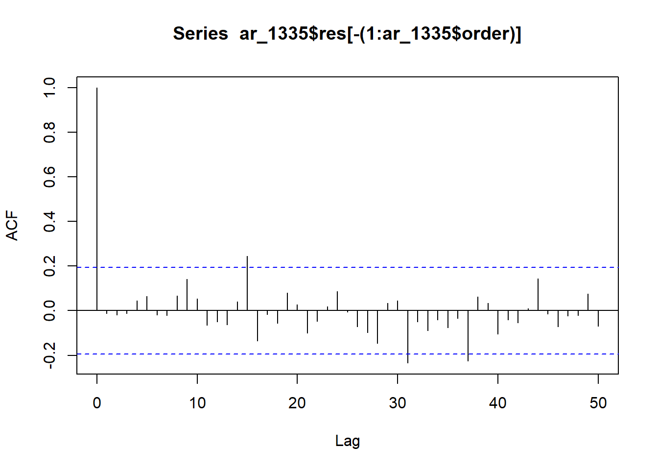
The correlogram of residuals has a few marginally significant lags (around 15 and between 30-40). The AR(6) model is a relatively good fit for the time series.
Regression
Deterministic trends and seasonal variation can be modeled using regression.
Linear models are non-stationary for time series data, thus a non-stationary time series must be differenced.
diff <- window(ts_1335, start = 1991)
## Warning in window.default(x, ...): 'start' value not changed
head(diff)
##            Jan       Feb       Mar       Apr May Jun Jul Aug Sep Oct       Nov
## 1991                                                                 0.2297590
## 1992 0.2754533 0.2595562 0.1728301 0.2423733
##            Dec
## 1991 0.1954429
## 1992
lm_s1335 <- lm(diff ~ time(diff)) # extract the time component as the explanatory variable
coef(lm_s1335)
##   (Intercept)    time(diff)
## -11.040746179   0.005700586
confint(lm_s1335)
##                     2.5 %     97.5 %
## (Intercept) -31.137573143 9.05608078
## time(diff)   -0.004366695 0.01576787
acf(resid(lm_s1335))
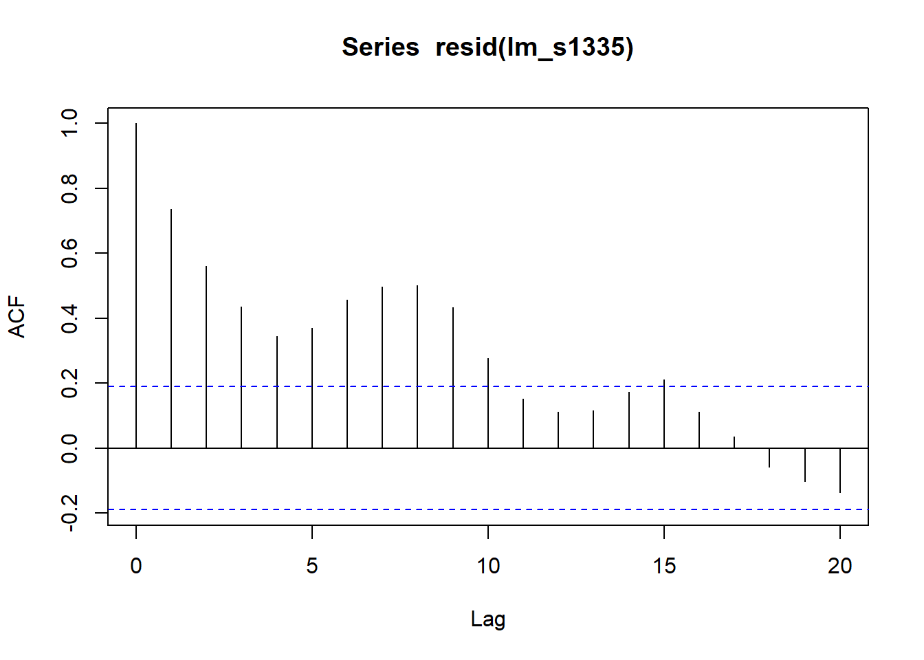
The confidence interval does not include 0, which means there is no statistical evidence of increasing Compound X in the atmosphere. The ACF of the model residuals are significantly positively autocorrelated meaning the model likely underestimates the standard error and the confidence interval is too narrow.
Adding a seasonal component
Seas <- cycle(diff)
Time <- time(diff)
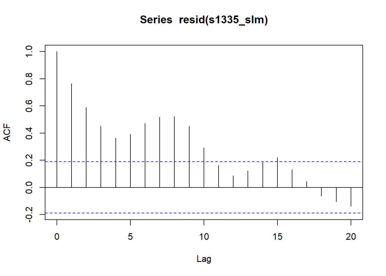
s1335_slm <- lm(ts_1335 ~ 0 + Time + factor(Seas))
coef(s1335_slm)
## Time factor(Seas)1 factor(Seas)2 factor(Seas)3 factor(Seas)4
## 0.005756378 -11.122691112 -11.131937489 -11.162273796 -11.124295885
## factor(Seas)5 factor(Seas)6 factor(Seas)7 factor(Seas)8 factor(Seas)9
## -11.155275762 -11.202207940 -11.174639108 -11.139997655 -11.123771124
## factor(Seas)10 factor(Seas)11 factor(Seas)12
## -11.171495571 -11.139425944 -11.179592661
acf(resid(s1335_slm))
Generalised Least Squares
Generalised Least Squares model can account for some of this autocorrelation.
From 5.4 of Cowpertwait & Metcalfe, 2009:
Generalised Least Squares can be used to provide better estimates of the standard errors of the regression parameters to account for the autocorrelation in the residual series.
A correlation structure is defined using the cor argument. The value is estimated from the acf at lag 1 in the previous correlogram. The residuals are approximated as an AR(1).
library(nlme)
##
## Attaching package: 'nlme'
## The following object is masked from 'package:forecast':
##
##     getResponse
## The following object is masked from 'package:dplyr':
##
##     collapse
gls_s1335 <- gls(ts_1335 ~ time(ts_1335), cor = corAR1(0.7))
coef(gls_s1335)
##   (Intercept) time(ts_1335)
##   -27.9996694     0.0141997
confint(gls_s1335)
##                      2.5 %      97.5 %
## (Intercept)   -87.94374736 31.94440847
## time(ts_1335)  -0.01582862  0.04422801
acf(resid(gls_s1335))
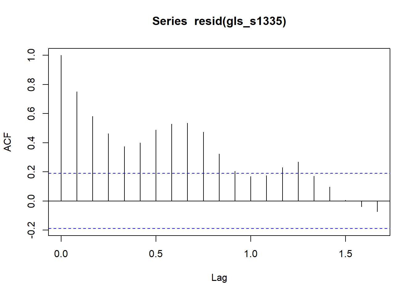
The confidence interval still includes 0 and the acf of the model residuals still have significant autocorrelation.
Autoregressive Integated Moving Average (ARIMA)
Autoregressive integrated moving average models define the model order (p, d, q).
Cookbook R explains it as:
p is the number of autoregressive coefficients, d is the degree of differencing, and q is tne number of moving average coefficients.
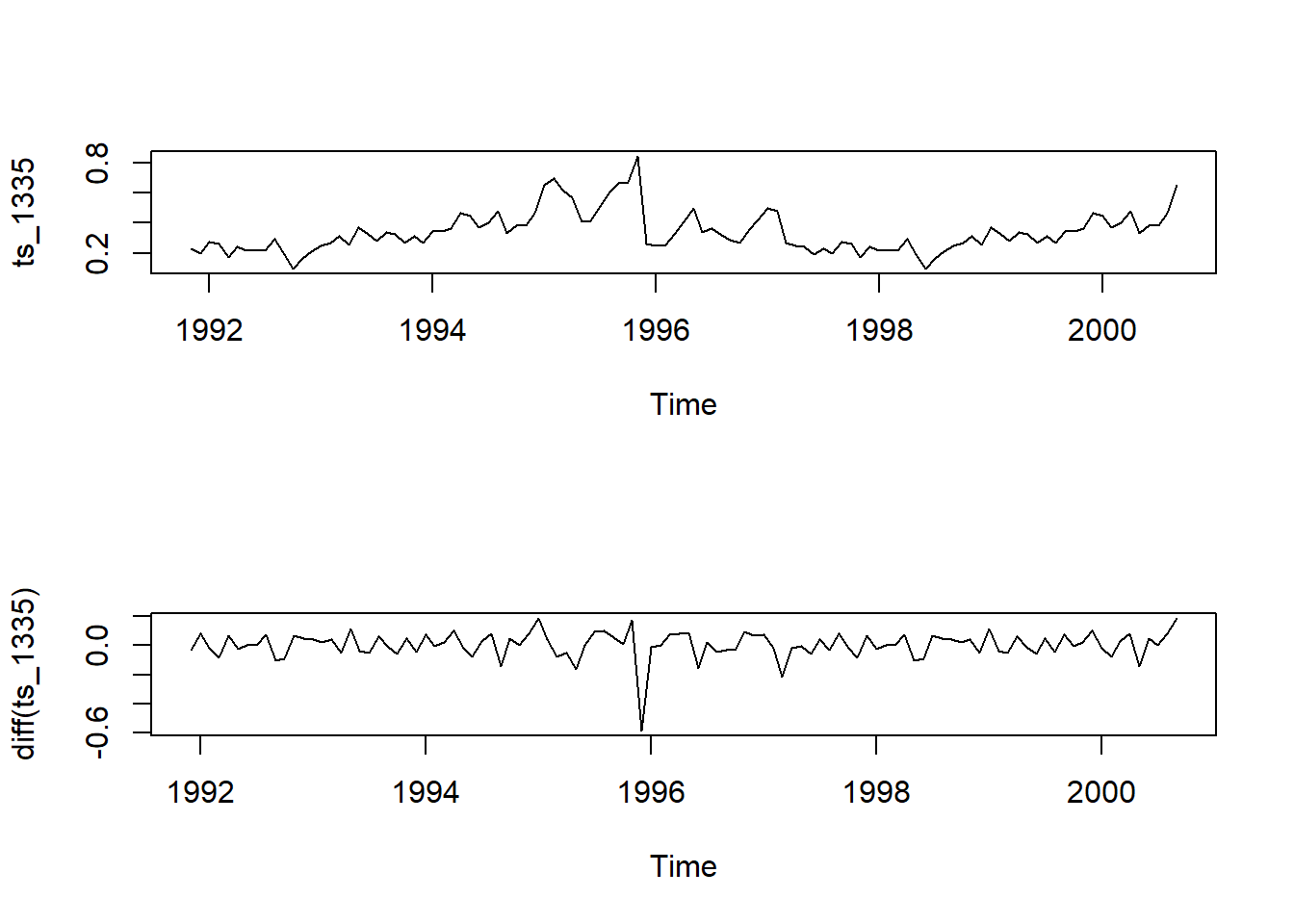
par(mfrow = c(2,1)) # change window so 2 rows, 1 column of plots
plot(ts_1335)
plot(diff(ts_1335))
arima_1 <-  arima(ts_1335, order = c(6,1,12))
## Warning in arima(ts_1335, order = c(6, 1, 12)): possible convergence problem:
## optim gave code = 1
arima_1
##
## Call:
## arima(x = ts_1335, order = c(6, 1, 12))
##
## Coefficients:
## Warning in sqrt(diag(x$var.coef)): NaNs produced
##          ar1      ar2      ar3      ar4     ar5      ar6      ma1    ma2
##       0.3101  -0.1672  -0.2606  -0.5937  0.3171  -0.3346  -0.6401  0.161
## s.e.  0.4987      NaN   0.1375   0.2446  0.3642      NaN   0.5091    NaN
##          ma3     ma4      ma5     ma6      ma7     ma8     ma9    ma10     ma11
##       0.2277  0.3546  -0.7157  0.5324  -0.1141  0.0339  0.0639  0.0186  -0.2655
## s.e.  0.3045  0.1810   0.2855     NaN      NaN     NaN     NaN  0.1282   0.2167
##         ma12
##       0.2497
## s.e.  0.1244
##
## sigma^2 estimated as 0.005943:  log likelihood = 119.27,  aic = -200.54
acf(resid(arima_1), lag = 50)
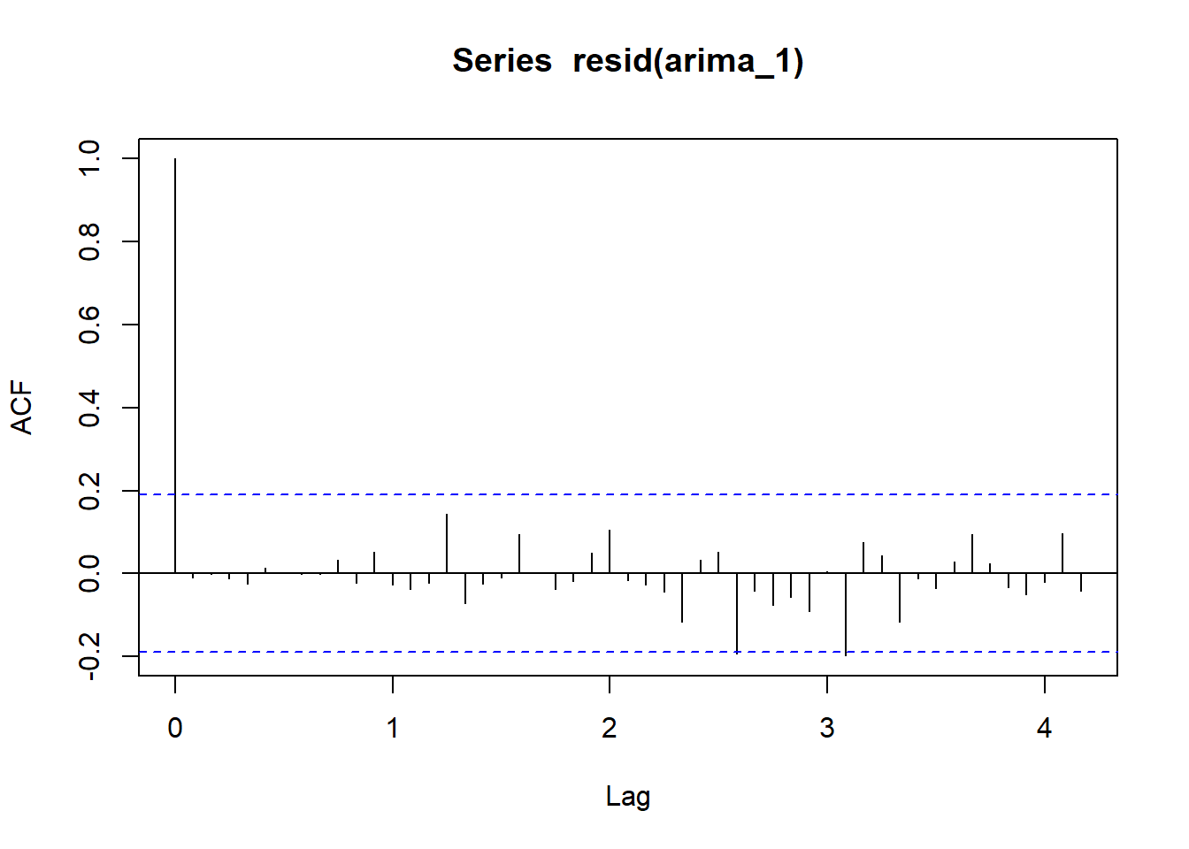
Let’s run a model with order(1, 1, 1) and compare AIC.
arima_2 <-  arima(ts_1335, order = c(1, 1, 1))
arima_2
##
## Call:
## arima(x = ts_1335, order = c(1, 1, 1))
##
## Coefficients:
##          ar1      ma1
##       0.5484  -0.8285
## s.e.  0.1300   0.0795
##
## sigma^2 estimated as 0.007826:  log likelihood = 106.51,  aic = -207.01
acf(resid(arima_2), lag = 50)
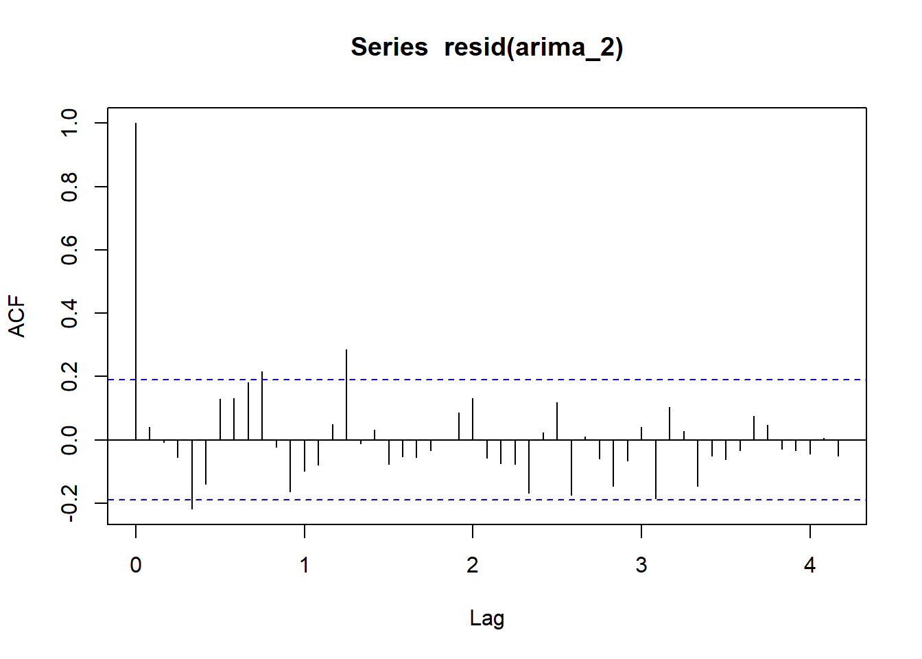
The second model had a lower AIC. Let’s use the forecast::auto.arima() function from the forecast package to search for the best p, d, q.
arima_3 <- auto.arima(ts_1335, seasonal = FALSE, max.p = 20, max.q = 20)
arima_3
## Series: ts_1335
## ARIMA(1,0,0) with non-zero mean
##
## Coefficients:
##          ar1    mean
##       0.7719  0.3452
## s.e.  0.0637  0.0362
##
## sigma^2 = 0.007892:  log likelihood = 107.77
## AIC=-209.54   AICc=-209.31   BIC=-201.52
acf(resid(arima_3), lag = 50)
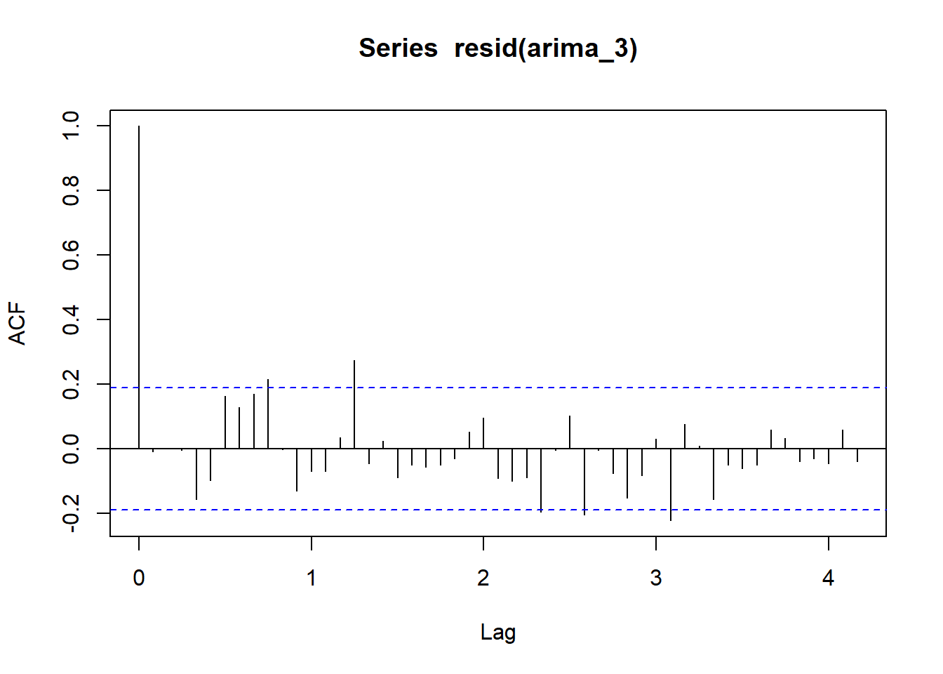
autoplot(ts_1335) # plot the time series
Seasonal ARIMA
A seasonal component can also be added to ARIMA. The default for auto.arima() includes the seasonal component.
sarima <- auto.arima(ts_1335)
sarima
## Series: ts_1335
## ARIMA(1,0,0) with non-zero mean
##
## Coefficients:
##          ar1    mean
##       0.7719  0.3452
## s.e.  0.0637  0.0362
##
## sigma^2 = 0.007892:  log likelihood = 107.77
## AIC=-209.54   AICc=-209.31   BIC=-201.52
acf(resid(sarima), lag = 50)

The addition of the seasonal component improves the AIC and the correlogram is close to the ‘white noise’ standard.
Resources
Check out tidyverts, tidy tools for time series!
Resources used to compile this session included:
- Introductory Time Series with R by Paul Cowpertwait and Andrew Metcalfe, Springer 2009.
- Ch 14 Time Series Analysis in R Cookbook, 2nd edition, by JD Long and Paul Teetor. Copyright 2019 JD Long and Paul Teetor, 978-1-492-04068-2
- Time Series Analysis with R by Nicola Righetti
- Applied Time Series Analysis For Fisheries and Environmental Sciences by Elizabeth Holmes, Mark Scheuerell, and Eric Ward.
- Time Series Analysis article by Selva Prabhakaran
- Working with Financial Time Series Data in R document by Eric Zivot.